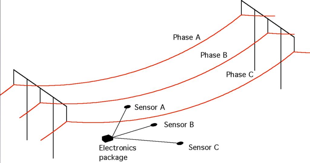
One of the grid enhancing technologies is Dynamic Line Rating (DLR). For the application of dynamic line rating, often sensors are used to monitor the behaviour of conductors. But how does this sensor monitor the transmission line conductor?
The sag of transmission line conductors is one of the most important aspects to monitor for a transmission system operator, because it is directly related to both safety and the loading current of an overhead line. There are different sag monitoring options. But which one is best?
There are many different ways to monitor the sag. They all have their own features, but they also come with some disadvantages. We have listed the different techniques for you below. They are sorted by direct and indirect measurements. Indirect measurement of conductor sag means that the sag is calculated using a different conductor characteristic.
Direct sag measurements
The direct measurement of conductor sag can be performed from three different locations [01]:
- from the air (aerial),
- from the ground (terrestrial) and
- from the conductor.
There are many techniques and solutions described in literature, but for aerial and terrestrial measurement they all boil down to using camera’s, lasers or a combination of both. References to lasers often refer to LiDAR technology. One instance using sonar is also reported. In generic these methods provide a reasonable accuracy. It was found that the combination of camera and laser provides a higher accuracy.


For measurement on the conductor, the same sensing type is also used. In addition, literature also describes the application of 1 or 2 GPS receivers. If you want to go for a high accuracy, two differential GPS receivers provide the best result.
Indirect sag monitoring
Where the number of options to directly measure the sag is limited, the number of different indirect measurement options is huge [01]. We have listed them below in alphabetical order.
Carrier signal
Since the sag is an integral aspect of line geometry, any change in sag alters the line’s geometry [04]. In turn it affects the electrical and magnetic fields near the transmission line and modifies the power line carrier signal within the line. By measuring the variations in the power line carrier signal between two stations, the sag can be calculated. While it provides good accuracy and is based on a straightforward theory, it requires a power line carrier signalling system with two stations. This setup is complex and has high maintenance costs.
Magnetic field
The relationship between the sag and the magnetic field is defined by a simple formula [05]. Therefore this method can be applied for sag monitoring. When the current flows through the conductors, it will generate a magnetic field around the line which can easily be measured, typically using multiple sensors. If the current intensity is known, the distance can be calculated directly.

It should be noted though, that he magnetic field depends on the intensity of the current and the distance to the overhead line. This means that the current value needs to be known, because it is needed as direct input for the calculation. For the best result, the current amplitude (and phase angles) of all conductors in the overhead line shall be determined to also account for asymmetric effects.
Optical
Sag and tension affect the attenuation of optical fibres in transmission lines. Therefore, optical sensors can be utilized to detect the optical changes induced by sag and calculate sag through these relationships. This measurement can be performed over a long length using one sensor. The sensor can be placed on the fibre in an optical ground wire (OPGW), or even more ideal: in a phase wire that has glass fibres incorporated in them.
This sag monitoring option is getting more popular and is commercially offered by multiple companies. They may have different techniques applied in their solution.

Phasor measurement units (PMU)
PMUs record current, voltage, and frequency values with very precise GPS time-stamping. If you have those readings from 2 sides of an overhead line, the line impedance can be calculated. Because the line impedance is temperature dependent, the PMU readings can be used to indirectly calculate sag. This also means that the user will receive one estimation for the complete line at once. The temperature variation along the line is unknown, meaning that hotspots are not visible. For good accuracy, the user is advised to take the inaccuracy of the current and voltage transformers into account.
Radio frequency (RF)
Path loss in radio frequency communications is influenced by the distance between the transmitter and the receiver, as the radio signal weakens with increasing distance. Therefore, knowing both the received signal strength and the transmitted signal strength allows for the calculation of the distance between them.
For sag estimation in an overhead line scenario, where the transmitter is positioned in the middle of the span and the receiver is on the ground, the sag can be estimated using the calculated distances derived from the received signal strengths.
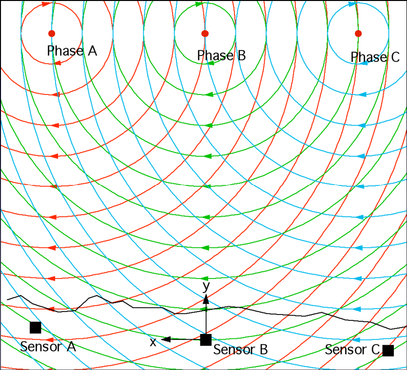
Space potential (electric field)
The potential between the phase conductors, shielding wires and ground result in a space potential that can be measured. To properly determine the sag from here, you will first need to solve the electromagnetic field distribution and establish the relationship between the field source parameter and the spatial EM field distribution value.
Surface acoustic wave
Surface acoustic wave (SAW) elements are used as narrowband filters, RFID tags, and sensors for measuring torque, force, temperature, and tension. These sensors can also measure temperature in transmission lines using a radio link for connection. A high-frequency electromagnetic wave is transmitted to the sensor, where it is converted into an acoustic surface wave by the sensor’s transducer. This wave propagates along the crystal’s surface and is reflected by integrated reflectors, whose positions change due to thermal expansion. The reflected signals, which depend on temperature, are converted back to high frequency and sent to the receiving antenna. Algorithms extract sensor ID and temperature information from these reflected signals by analysing their time position and phase relation.
Tension
Sag is inversely proportional to the tension in the overhead line. So if you measure the tension, you are able to estimate the sag. The first sag measurements were based on this technique, which is pretty straightforward. It also allows the user to install sensors in between the conductor and the towers, which may be quite labour intensive.
Temperature – current
Instead of the sag-tension relationship, the sag-temperature relationship is often used to calculate the sag too, as thermal expansion is one of the main reasons of sagging. It is also the key parameter for dynamic line rating and is closely related to the current in the overhead line.
The temperature–current methods basically use the sag-tension formulas, but through the parameters of temperature and current to calculate the sag more indirectly.
Tilt
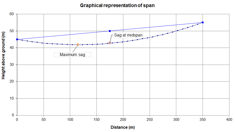
The sag is also a function of the angle of tilt of the line at (or close to) the tower. The angle of tilt can be derived from the catenary equation using the geometry of a sagged line, as is visible in figure X Therefore, if you measure the angle of tilt you can estimate the sag.
Vibration
Overhead transmission lines may appear to be quite static, but actually they are in constant vibration due to the wind and actions of other (external and internal) loads on the line. Like a guitar string, the conductor has a certain frequency that depends on the length and tension between the two towers. So if you measure the vibration, you can calculate the length of the conductor, and therefore determine other parameters, such as the sag.
It should be note that the vibration method effectively leverages the relationship between sag and vibration period or frequency to provide highly accurate sag calculations. This relationship is straightforward, requiring only the loading parameter or a constant. However, this simplicity comes at the expense of general applicability. For instance, varying temperatures result in different frequencies, necessitating different constants. Consequently, the method must be recalibrated whenever conditions or span change. Another drawback is that its accuracy diminishes when the vibration is minimal or the line remains stationary.
Summary of sag monitoring options
The following table provides a summary of the different techniques that can be used to measure the sag of an overhead line.
| Accuracy | Cost | |
| Carrier signal | L | H |
| Magnetic field | H | L |
| Optical | H | H |
| PMU | L | H |
| RF | L | L |
| Space potential | H | L |
| Surface acoustic wave | H | H |
| Tension | H | M |
| Temperature – current | L | M |
| Tilt / slope | H | M |
| Vibration | H | M |
References
[01] Survey of line monitoring
[02] www.researchgate.net/Various-dynamic-thermal-rating-DTR-sensors-a-Weather-monitoring-station
[03] https://discuss.px4.io/t/vtol-fixed-wing-drone-lidar/27297
[04] https://ieeexplore.ieee.org/abstract/document/4402890
[05] https://halverscience.net/about_halverson/Promethean/files/Promethean_EPRI_08_slides.pdf
[06] https://www.prismaphotonics.com/our-technology/