Here we describe the value of the measurement data and estimated geo-electric soil models as provided by the DINO loket, specifically for the application in high voltage engineering. First it is important to understand what data is provided by DINO loket. Then, equally important, is to understand how measurement data can be processed to a soil model. And finally, there is the question: how do the choices in the process influence the outcome of my calculations? We try to provide insight using an example.
Which three steps are needed to form a 1D geo-electric soil model?
The process to go from measurements to 1D soil model consists of 3 steps:
- Measurements; by injecting a current and measuring the voltage a resistive value can be determined. Simply following Ohm’s law.
- Conversion; the resistive values can be converted to values for apparent soil resistivity, per electrode configuration
- Inversion; a curve can be fitted through the converted data to estimate the soil characteristics and layer buildup.
This leads to a 1D soil model, where each horizontal layer is described by the thickness and resistivity value.
Note: a 1D model is a simplified representation of the soil at the location of the measurement. It assumes a perfectly horizontal layering with a uniform resistivity distribution throughout the layer. This is a simplification that is normally justified by rounding the numbers conservatively. However, depending on the application, different choices can be made.
What is provided by DINO loket?
Unless you are lucky enough to have access to a database with measurement data, you would probably need to perform measurements yourself. In the Netherlands such a database (with freely accessible data) is available. The DINO loket provides thousands of VES/Schlumberger and VES/Wenner measurements throughout the whole country. In addition there is also a huge amount of other measurement results (such as bore-hole information) available. Some of these measurements date back to 60 or 70 years ago.
The data was initially intended for use in the geological sciences. This means that DINO loket information was never directly meant to be used in high voltage engineering. However, it has proven to be a very useful source.
What information is in the Schlumberger measurement files?
All the Schlumberger measurement files contain the values of the apparent soil resistivity (the converted data) and most of the files also have a 1D model description in them (inverted data). In most files there is no raw measurement data (voltage and current values), this can only be found in a few.
Next to that, the files also have an unique number and contains coordinates, the data when the measurements were performed and an indication about the model interpretations (up to which depth the data provides information and how well the inversion was done, if a 1D model is provided).
Check this page to get an idea of the data that is provided.
How should I interpret the Schlumberger measurements?
The measurements are typically performed over a length of several hundreds of meters. This provides information up to a significant depth, which is very useful. There are a few points of attention:
- Seasonal dependency of the top layer(s); the resistivity of the top layers may vary over time, depending on the weather.
- Double measurement points; the Schlumberger method is especially convenient if large measurement profiles are applied, since the middle two electrodes can remain at the same position during the measurements… unless the measurement accuracy is affected. In that case, the electrode spacing of the voltage probes needs to be increased. If you see multiple measurement points for a specific electrode arrangement, this means that the inner electrodes have been re-configured. In that case we advise to take the last measurement point that is measured. Note: the measurements taken just before this one may be less accurate.
- Maximum depth; the inversion method assumes an infinite depth for the lowest layer to fit the curve through the measurement data. This is a mathematical necessity in the process. However, this does not mean that you know all about the very deep layers. In case of a ‘good fit’ the measurements typically represent a depth equal to the electrode spacing. In case of a ‘fair fit’, you need to be careful with the lower layers.
- The thickness and resistivity values of the lower layers can be estimated during inversion, but the deeper you look, the wider the range of the values for these properties may be to achieve a fit. This is especially the case if the number of layers is large (much variety throughout the soil).
These points justify the rounding of values, especially for the shallow and deep layers. There is not one method that is always right. You need to know the effect of the choices that you make. Therefore, let’s take an example!
Example of interpretation of DINO loket Schlumberger measurement
We have randomly selected a measurement profile from DINO loket, the one with identity NITG-nr: W17H0003. DINO loket has made the interpretation of a 7-layer soil model with the following characteristics.
| Layer | Thickness (m) | Apparant soil resistivity (Ohm.m) |
| 1 | 1 | 170 |
| 2 | 4 | 80 |
| 3 | 20 | 170 |
| 4 | 15 | 80 |
| 5 | 50 | 150 |
| 6 | 50 | 100 |
| 7 | inf | 5 |
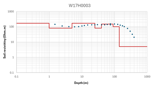
As you can see, all layer thickness values are rounded to integers. This means that you will never see a layer thickness of less than 1m. Also, in many cases, the layer resistivity values appear to be rounded to the nearest five for values up to 100 Ohm.m and to the nearest ten for values above that.
It should be noted that not much information about this data is provided. The measurements date from a long time ago, is not complete regarding electrode spacing and the options for automized processing using computer algorithms were limited in the past. Therefore, we assume that the inversion of the data may not be optimally performed.
Example of interpretation of DINO loket Schlumberger measurement
Re-investigation of the data was done using an automized version of our online tool, which is based on the original program from DINO (using a simplified method to make an interpretation of the data), looking at different amounts of layers (4 to 7 layers). The outcome of the analysis is displayed in the following tables and graphs.
| Layer | 7 layers | 6 layers | 5 layers | 4 layers | ||||
| Thickness (m) | Resistivity (Ω·m) | Thickness (m) | Resistivity (Ω·m) | Thickness (m) | Resistivity (Ω·m) | Thickness (m) | Resistivity (Ω·m) | |
| 1 | 0.92 | 172 | 0.94 | 171 | 0.78 | 194 | 0.62 | 186 |
| 2 | 4.00 | 79.3 | 4.10 | 79.1 | 2.24 | 78.1 | 7.89 | 100 |
| 3 | 8.56 | 234 | 7.63 | 255 | 38.6 | 136 | 104.6 | 174 |
| 4 | 2.21 | 10.3 | 2.22 | 10.3 | 36.1 | 374 | inf | 0.86 |
| 5 | 19.1 | 847 | 19.2 | 866 | inf | 1.01 | ||
| 6 | 35.1 | 13.8 | inf | 1.12 | ||||
| 7 | inf | 0.45 | ||||||
| Linear RMS error | 2.85 | 2.91 | 4.3 | 7.6 | ||||
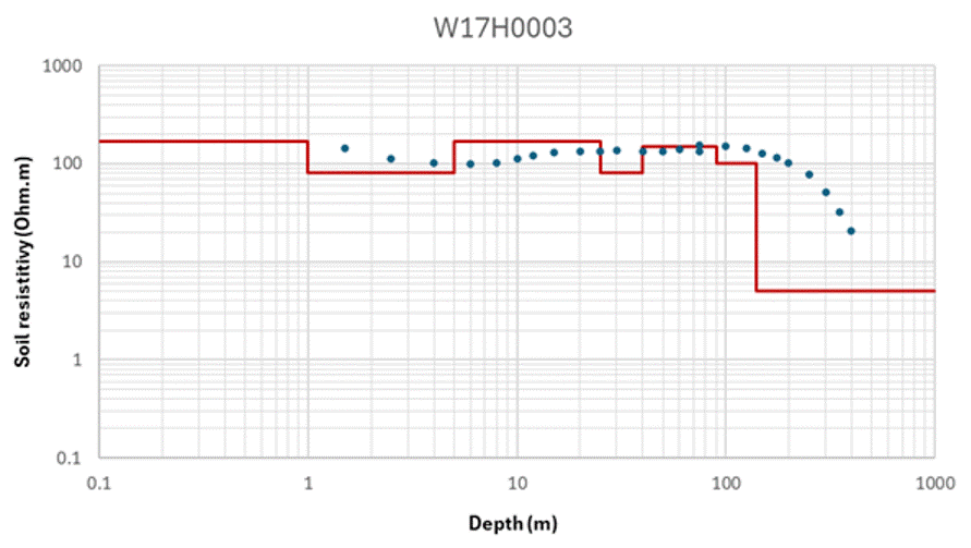
The comparison of the 7 layer model from the recent analysis with the DINO model shows the following.
- A rather good comparison of the resistivity values for the top two layers, with a slight difference due to the rounding effect.
- A rather large variation of the lower layers, where especially the bottom layer is surprisingly low.
Based on the RMS error and graphs a 5-layer model would seem to be a good choice. Let’s see what this does with the earthing resistance, soil potentials and touch voltage.
What is the influence of the 1D soil model on the earthing resistance and potentials?
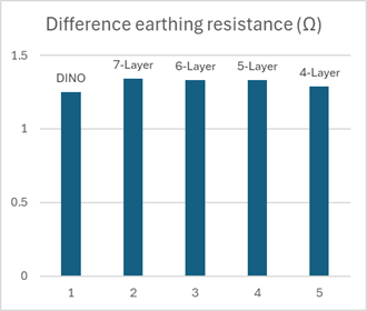
The earthing resistance, soil potentials and touch voltage are calculated for all 5 of the geo-electric soil models, looking at a simple earthing grid consisting of a 10m mesh and 4 vertical electrodes at the corners.
The earthing resistance lies between 1.251 Ohm and 1.341 Ohm. Using the 5-layer soil model as a reference, the value for the DINO loket soil model is 6.5% lower. There is hardly any difference between the different layer models, except for the 4-layer model. For the purpose of calculating the earthing resistance value, the 4-layer model seems to be over-simplified.
| DINO | 7-Layer | 6-Layer | 5-Layer | 4-Layer |
| 1.251 Ω | 1.341 Ω | 1.332 Ω | 1.332 Ω | 1.288 Ω |
| -6.5% | 0.7% | 0.0% | 0.0% | -3.4% |
The soil potentials have also been calculated. Here, the same trend is visible. There is hardly any difference between the different layer models, except for the DINO loket soil model and 4-layer soil model.
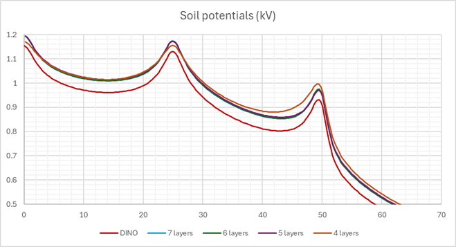
Then, the final aspect that is of importance is how the touch potential is influenced by this. The touch potential is the difference between the EPR of the grid and the soil potential at 1m distance from any touchable object. You can find a graphical representation in the graph below.
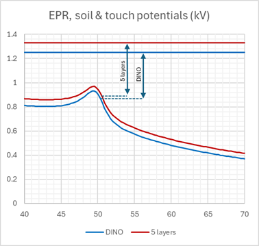
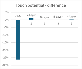
Comparison of the touch voltages of all the cases shows that the selection of the amount of layers is hardly impacting the final values of the touch voltages (differences limited to about 1%). For the 4-layer model this means that the difference of the earthing resistance and the soil potential are canceling each other out. The calculated touch voltage using the DINO loket model is more than 25% lower. This is a significant difference.
Conclusion
Based on this analysis we can conclude that it is possible to reduce the amount of layers in the interpretation of a soil model, as long as the error stays within acceptable limits. This will have limited influence on the outcome of the calculations. It is always advised to double check the analysis performed by others, especially if it is unknown what exact method is used. And, depending on the purpose, the user may want to use rounding of the numbers to add some conservatism.